Did You Know? #10 You can download NASA and USGS Data for Free?

That you can download Landsat imagery for free? On August 17th the 1 millionth Landsat image was downloaded since the Landsat imagery archive was made available to the public last October in 2008 at no cost. The selected image was that of the Grand Canyon captured by the Landsat 5 sensor and can be seen below.

You can download your own images for use in GIS programs from:

The USGS GloVis is a fun way to preview imagery or browse the globe, but if you need lots of data for a specific area the USGS Earth Explorer will probably suit your needs a little better.

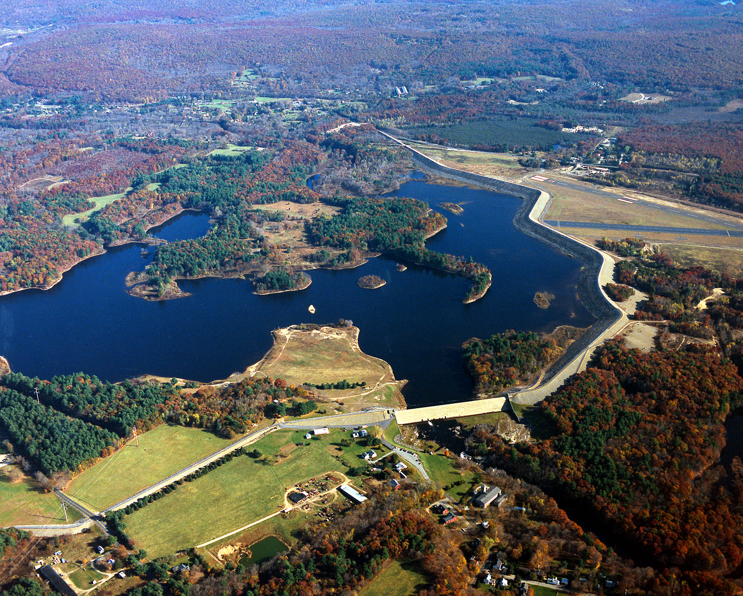
If you don’t really need GIS data for analysis but think the Earth is beautiful, check out Earth as Art from the Goddard Space Flight Center. Most of the images are captured by Landsat 7 and would dress up any room. Below is one of my favorites:

Can you guess the location?

Did you Know? #9 The changing geography of Connecticut through topographic maps.

People often have the misconception that geographers and cartographers are not relevant because “everything has been mapped”. But the landscape is always changing! Here are some examples of significant changes in the state over the past century.

Click on the images to enlarge them.

Ocean Beach, New London: Prior to 1938, the maps show homes along with two bridges in the area. However, the hurricane of 1938 destroyed most of the homes and one of the bridges. The Ocean Beach Area was changed to a park after the hurricane, as seen in 1958 topographic map. See photographs of what Ocean Beach looked like in 1923 and now.

Ocean Beach in 1938

Ocean Beach in 1958

Downtown Hartford: In the early 1950s, Downtown Hartford looked very different without interstate highways going through the city. Interstate 84 was built along the city’s major rail lines. After the construction of I-84, much of the Park River, found near the state capitol and Bushnell Park, was diverted into underground channels.

Downtown Hartford in 1952

Downtown Hartford in 1984

Mansfield Hollow, Mansfield: Mansfield Hollow Dam was built in 1952 by the Army Corps of Engineers to control flooding in the area. The large reservoir was created by damming the Natchaug River, which flooded a swampy area known as Turnip Meadow.

Mansfield Hollow in 1943

Mansfield Hollow in 1984

The Mansfield Hollow Area is shown below

Map of the Week! #4 Paris from Charles V to Charles IX

The title of this weeks featured map is:

Paris depuis Charles V jusqu’a Charles IX, d’après le plan de l’Abbaye St. Victor.
OR

Paris from Charles V to Charles IX, after the plan of the Abbey St. Victor.

That’s quite a long time period. In fact, the end of Charles V reign is dated at 1380 and the beginning of Charles the IX reign is dated at 1560. The additional information in the title referencing that it is after the plan of Abbey St. Victor gives us little help in narrowing down the dates of the map as the abbey was formed circa 1113. Also of note is that this map was published with the text “Tableau de Paris” By Louis-Sébastien Mercier in 1893. This is surely a later revised edition as Louis-Sébastien Mercier passed away in 1814.

To read an edition of this work look below to the embedded Google book. The edition is in French but if you copy the URL of the book and paste it in Google’s Translate tool you should be able to read it in English. (Tip: Set the text to “Plain Text” located in the upper right before translating)

Important features located on the map include Nostre Dame Cathedral now spelled Notre Dame:

St. Victor Abbey:

La Bastille, an icon of royal power that was stormed at the beginning of the French Revolution:

St. Eustache Cathedral with a pipe organ numbering ~8000 individual pipes rivaling the pipe organ in Notre Dame. For photos of St. Eustaches stained glass windows click here.


And Porte Saint-Denis, a fortified gate in the walls of old Paris.

Also for fun, see how many windmills you can find on the map here’s an example:

Did You Know? #8 Tracking Hurricane Bill

You can track Hurricane Bill and other hurricane activity in the Atlantic and Pacific Oceans at the National Weather ServicesNational Hurricane Center. You can also subscribe to a RSS feed that will automatically update you on changes in the storms status and provide you with GIS Shapefiles.

In 1938 A large hurricane made landfall in New England , visit the following resources for more information:

PBS
NOAA Coastal Services Interactive Map (GIS Data Download)
The University of Connecticut’s 1938 Hurricane Story
The Connecticut State Library 1938 Aerial Photos

Map of the Week! #3 Hartford in 1640 and 1893

Today’s featured map was made in 1838 and shows landowners in Hartford in 1640, shortly after the city was founded. Initially, a pastor named Thomas Hooker led a group of about 100 people from Cambridge, Massachusetts to Connecticut to form a new colony. They chose present day Hartford as their new settlement site.

In 1639, government officials of Connecticut colony, including Thomas Hooker and John Haynes, created a document called the “Fundamental Orders of Connecticut.” It is arguably the first written constitution in Western society, and helped give Connecticut the nickname of “the Constitution State”. The document emphasized individual rights and democracy.

The second map comes from the Connecticut State Atlas in 1893. The 1893 street network in Hartford is generally the same as today, but the river going through the southern part of the city (called the Little River in the historic maps, now called the Park River) is completely removed from maps and aerial photographs today. So what happened to it? In the 1940s, the Army Corps of Engineers rerouted the river through underground concrete channels in an effort to control flooding in Downtown Hartford. Click below to view a recent New York Times article about the underground Park River.

http://www.nytimes.com/2003/07/31/nyregion/paddling-hartford-s-scenic-sewer-abused-underground-river-up-close-noxious.html

The screen below shows the historic maps from 1640 and 1893, as well as recent aerial photos. Click the box that says “Famous Historical Residents” in the upper right of the screen to view where famous early Hartford residents lived in 1640.

List of landowners and corresponding land parcel numbers for 1640 map (click to enlarge):

To view the 1640 map in flickr, click here: http://www.flickr.com/photos/uconnlibrariesmagic/3836896031/

To view the 1893 map in flickr, click here:
http://www.flickr.com/photos/uconnlibrariesmagic/3837687450/

Links about the early settlers of Hartford:
http://www.hartfordhistory.net/faq.html

http://en.wikipedia.org/wiki/History_of_Hartford,_Connecticut

Did You Know? #6 Raster Vs. Vector

Geographic Information Systems (GIS) primarily use two categories of digital data: 1) Raster Data and 2) Vector Data.
Raster Data:
Raster Data portrays real world data as a matrix or a grid of cells (see Figure #1). Raster data is very good at storing continuous data (for example: precipitation, temperature, and elevation). Each cell stores information numerically, usually between 0-255 and has a geographical location. A weakness of raster data is that the cells are squares and most real world information doesn’t fit into a perfect square(See Figure#2). So sometimes a map made with satellite imagery will either underestimate or overestimate a land cover type.

Vector Data:
Vector Data portrays real world data as a point, line or polygon. Vector data is very good at storing discrete data (for example: political boundaries, rivers, lakes, land parcels, and streets). Each point, line, or polygon is called a feature and has a unique ID# (see Figure #2). Attribute information can be added to each feature in geographical space. A weakness of vector data is that it sometimes needs great amounts of processing power to run a complex analysis.
Below are links to examples of raster (Source: ESRI) and vector data (Source: CT DEP, MAGIC)
Click to view an example of vector data (point features):
Click to view an example of vector data (polygon features):
Click to view an example of vector data (Line features):

Did you Know? #5 Monitoring Climate Change

The discussion about global warming and climate change has largely focused on the increasing amounts of carbon dioxide released in the atmosphere. But how do we know this? One of the major carbon dioxide monitoring stations is located in an unlikely place; near the top of a 14,000 foot volcano on Hawaii’s Big Island.


Mauna Loa Volcano, Hawaii

Mauna Loa Observatory is found on the Mauna Loa volcano at an elevation of about 11,000 feet. Why collect data about carbon dioxide levels on top of one of the largest volcanoes in the world? Mauna Loa’s remote location and high elevation ensures that carbon dioxide measurements are the most accurate possible since they are not greatly affected by major sources of air pollution in Asia, America, and Europe.

Carbon dioxide measurements were first taken by Charles Keeling in 1958. Since then, the amount of the gas in the atmosphere has steadily increased from 315 parts per million to 385 parts per million.

View Larger Map

NOAA’s Mauna Loa Observatory

The tall tower takes carbon dioxide measurements at the observatory

Keeling’s graph of carbon dioxide levels, often called the Keeling Curve. The curve’s annual fluctuations are due to plants in the northern hemisphere absorbing carbon dioxide in the summer and then releasing it during the winter as deciduous trees lose their leaves.

How in the World? #3 – Georeferencing

In our first “How in the World” we showed you how a paper map is scanned and converted into a digital image. The map has geographic information drawn on it, but once it’s scanned it’s still just a picture. How can we place the image so that its extent is defined in physical or geographical space? We georeference it, that’s how!

Remember our Map of the Week featuring Sachemdoms, villages and trails? It began as a paper map, now it’s a digital masterpiece! All it took was:

  • A vector file (most commonly referred to as a Shapefile or Coverage)of Connecticut with latitude and longitude information stored within,
  • Our scanned Image,

  • And GIS Software.

Basically, we display both images on the computer screen and stretch them so the boundaries match and then tack them in place. When we tell the software to save the original paper map image, it also saves the latitude and longitude information with it. This information allows us to use it in other GIS programs or Google Maps! Watch this video to see how we georeference a paper map!

IT’S MAGIC!
~Jeff